目次
はじめに
MATLABのfigureでプロットすると余白が大きい時があって、パワポに貼り付け後にトリミングをやっていた。
どうにかならんのかと思っていたが、同じ悩みを抱える人はいるようでAutomatically remove white space from figureのような質問がある。
その回答で示されていたのが、余白を最小限にしたプロットの保存およびコピーというページだった。
このなかで紹介されているのが大きく二つの方法だ。
一つがexportgraphics (copygraphics もあるが、これはクリップボードにコピーするだけ)を使う方法。 もう一つがtiledlayoutでコンパクトにするオプションを設定する方法。
tiledlayoutの場合は通常は二つ以上を配置する時に使う。
どれくらい違うかを確認してみた。
exportgraphicsを使う場合
こんな例の場合:
x = 0:pi/100:2*pi;
fig_handle_1 = figure(1);
plot(x, sin(x), 'LineWidth',2)
xlabel("$x$", "Interpreter","latex")
ylabel("$\sin (x)$ ", "Interpreter","latex")
ax = gca;
ax.FontSize = 18;
これを次のコマンドでpngに保存してみる。
saveas(fig_handle_1, "sine_curve.png")
exportgraphics(fig_handle_1, "sine_curve_2.png")
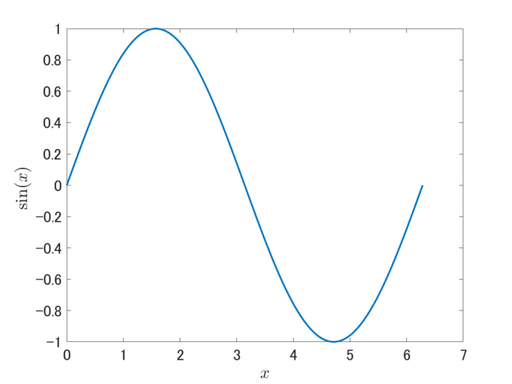
まずはsaveasで保存した場合。画像のサイズが分かるようにcssでgreen の borderを付けてある。
exportgraphicsで保存した場合
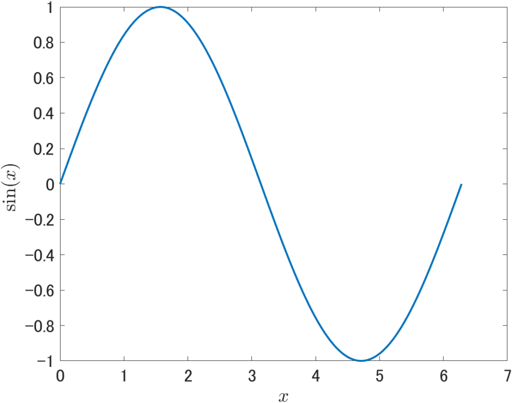
exportgraphicsを使うほうが、確かに余白が小さくなる。
tiledlayoutのオプションを指定する場合
次のような例:
%%
x = 0:pi/100:2*pi;
%%
figure_handle_2 = figure(2);
tiled_handle_1 = tiledlayout(2, 4);
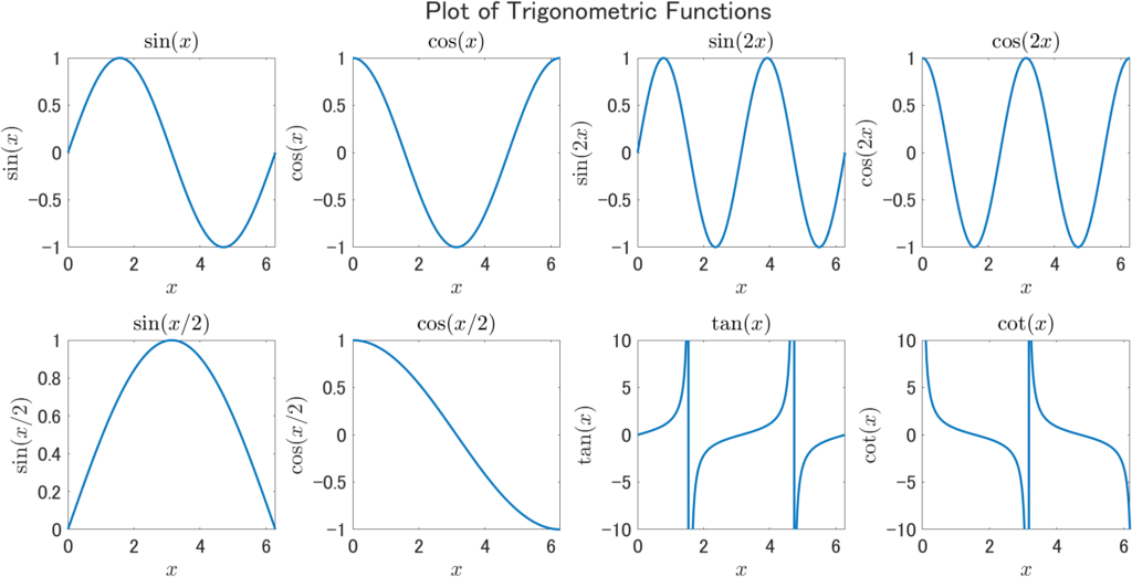
title(tiled_handle_1, "Plot of Trigonometric Functions")
tiled_handle_1.Title.FontSize = 24;
nexttile
plot(x, sin(x), 'LineWidth', 2)
xlabel("$x$", "Interpreter","latex")
ylabel("$\sin(x)$", "Interpreter","latex")
title("$\sin(x)$", "Interpreter","latex", "FontSize", 18)
ax = gca;
ax.FontSize = 18;
nexttile
plot(x, cos(x), 'LineWidth', 2)
xlabel("$x$", "Interpreter","latex")
ylabel("$\cos(x)$", "Interpreter","latex")
title("$\cos(x)$", "Interpreter","latex", "FontSize", 18)
ax = gca;
ax.FontSize = 18;
nexttile
plot(x, sin(2*x), 'LineWidth', 2)
xlabel("$x$", "Interpreter","latex")
ylabel("$\sin(2x)$", "Interpreter","latex")
title("$\sin(2x)$", "Interpreter","latex", "FontSize", 18)
ax = gca;
ax.FontSize = 18;
nexttile
plot(x, cos(2*x), 'LineWidth', 2)
xlabel("$x$", "Interpreter","latex")
ylabel("$\cos(2x)$", "Interpreter","latex")
title("$\cos(2x)$", "Interpreter","latex", "FontSize", 18)
ax = gca;
ax.FontSize = 18;
nexttile
plot(x, sin(x/2), 'LineWidth', 2)
xlabel("$x$", "Interpreter","latex")
ylabel("$\sin(x/2)$", "Interpreter","latex")
title("$\sin(x/2)$", "Interpreter","latex", "FontSize", 18)
ax = gca;
ax.FontSize = 18;
nexttile
plot(x, cos(x/2), 'LineWidth', 2)
xlabel("$x$", "Interpreter","latex")
ylabel("$\cos(x/2)$", "Interpreter","latex")
title("$\cos(x/2)$", "Interpreter","latex", "FontSize", 18)
ax = gca;
ax.FontSize = 18;
nexttile
plot(x, tan(x), 'LineWidth', 2)
xlabel("$x$", "Interpreter","latex")
ylabel("$\tan(x)$", "Interpreter","latex")
title("$\tan(x)$", "Interpreter","latex", "FontSize", 18)
ylim([-10 10])
ax = gca;
ax.FontSize = 18;
nexttile
plot(x, cot(x), 'LineWidth', 2)
xlabel("$x$", "Interpreter","latex")
ylabel("$\cot(x)$", "Interpreter","latex")
title("$\cot(x)$", "Interpreter","latex", "FontSize", 18)
ylim([-10 10])
ax = gca;
ax.FontSize = 18;
%%
saveas(figure_handle_2, "tiledLayoutEx01.png")
exportgraphics(figure_handle_2, "tiledLayoutEx01_2.png")
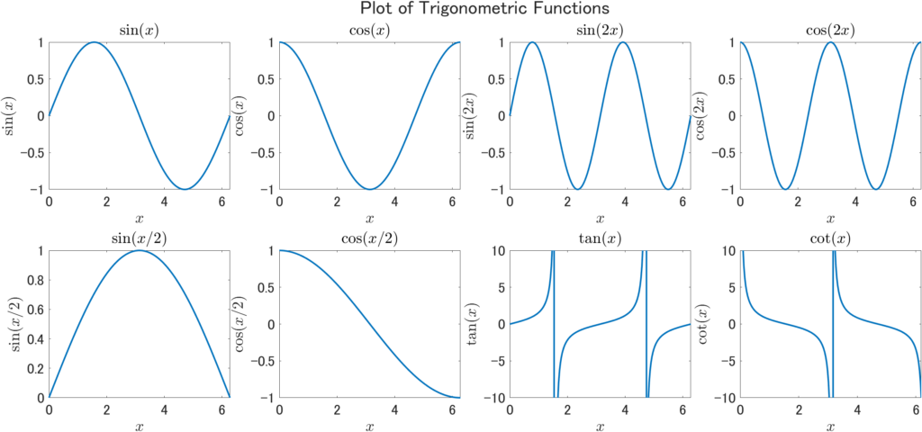
tiledlayoutのオプションを指定しない場合
上のコードのまま。具体的には下の部分だ。
tiled_handle_1 = tiledlayout(2, 4);
saveasで保存した場合

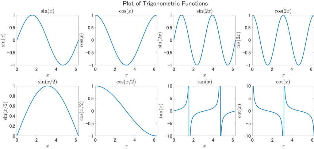
exportgraphicsで保存した場合
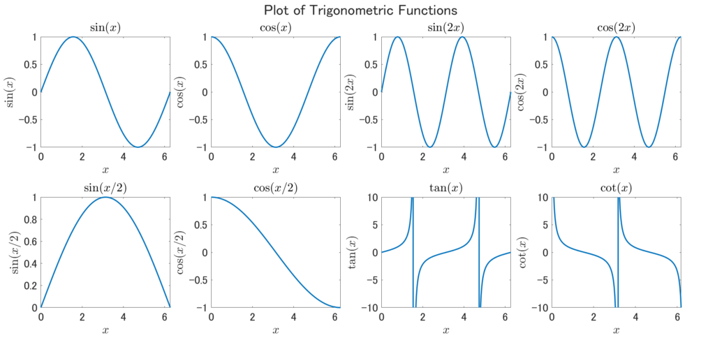
tiledlayoutのオプションで”tight”を指定した場合
具体的には下のようにオプションを指定する場合。
tiled_handle_1 = tiledlayout(2, 4, "TileSpacing","tight", "Padding","tight");
saveasで保存した場合
exportgraphicsで保存した場合
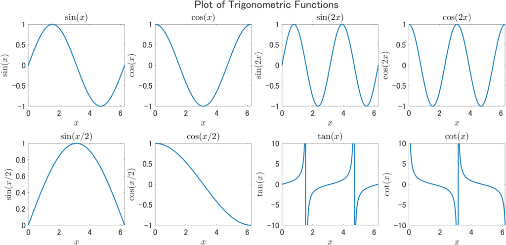
tiledlayoutのオプションで”compact”を指定した場合
具体的には下のようにオプションを指定する場合。
tiled_handle_1 = tiledlayout(2, 4, "TileSpacing", "compact", "Padding","compact");
saveasで保存した場合
exportgraphicsで保存した場合
tiledlayoutのオプションで”loose”を指定した場合
具体的には下のようにオプションを指定する場合。
tiled_handle_1 = tiledlayout(2, 4, "TileSpacing","loose", "Padding","loose");
saveasで保存した場合
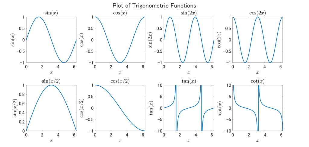
exportgraphicsで保存した場合

違い?
exportgraphicsの出力では、tiledlayoutのオプションの違いはかなり分かりづらい。
隣のグラフとの間隔が詰められる違いがある。
tightは詰まり過ぎな感じがするので、好みでcompactかlooseを選び、exportgraphicsで出力するのが良さそう。
長々調べておいて何だが、個人的にはexportgraphicsを使うのであればtiledlayoutのオプションは指定しなくても良いと思った。